Architecture of a First-Level Support Automation

How do you actually automate first-level customer support without the system collapsing into one big agent that nobody can debug? This post describes the architecture we landed on after iterating on a customer support system we built in production. It is a worked instance of the philosophy from Agentic vs Workflow-based AI: decompose the problem, let an LLM do only what only an LLM can do, and put code everywhere else.

The system takes a customer message — email, chat, whatever — and produces two things: a reply (possibly with attachments) and any tool calls needed to resolve the request (invalidate a voucher, file a reimbursement ticket, escalate to a human). Inbound attachments are normalised by a preprocessing layer before anything else runs.

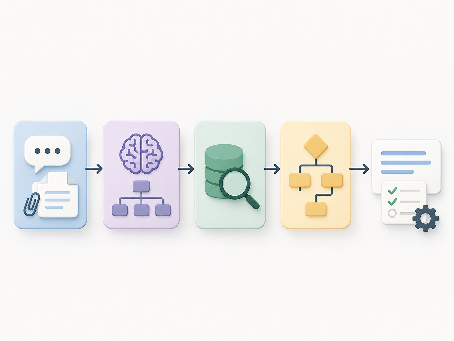
The pipeline has four steps, run as a DAG:

flowchart LR
    INPUT([Customer message<br/>+ attachments])
    INPUT --> S1[🤖 Intent recognition]
    INPUT --> S2[🤖 Information extraction]
    S2 --> S3[⚙️ Fetch]
    S1 --> S4[Plan generation]
    S3 --> S4[Plan generation]
    S4 --> OUT([Reply + tool calls])

Intent recognition and information extraction have no data dependency on each other, so they run in parallel. Fetch depends only on extraction, and plan generation pulls together the intent and the fetched records.

We will trace one message through all four steps. The running example throughout this post is:

Ich bin Kunde bei der Sparkasse Nürnberg, mein Name ist Max Müller, meine Partnerin Angelika Müller, Kontonummer ABCO1234. Wir kommen nicht mehr in unser Konto rein.

This message is realistic in three useful ways. The intent is slightly ambiguous (login problem? account locked? something else?). There are two people named and we do not yet know whose account is meant. And the account number contains the classic OCR-or-typing ambiguity between 0 and O — ABCO1234 could be ABC01234.

Step 1: Intent recognition

The job here is to classify the message into one of a small set of intents — cheaply enough that the downstream pipeline can branch on it.

We classify against a rooted DAG of intents — a single entry point, biased toward depth 2. The root has a handful of broad parent intents (“account access”, “payments”, “card services”, …) plus an explicit “other” parent. Most parents have a few sub-intents underneath, again plus an “other” within that parent. We run this as two LLM calls: first the parent intent, then — given the parent — the sub-intent from a constrained list. Both calls are simple Agent invocations with no tools and a typed output_type; see Type-Safe Hybrid Workflows with Pydantic AI for the mechanics.

flowchart TD
    R([Message])
    R --> P1[Account access]
    R --> P2[Payments]
    R --> P3[Card services]
    R --> POT[Other]

    P1 --> P1A[Login problem]
    P1 --> P1B[Password reset]
    P1 --> LOCKED[Account locked]
    P1 --> P1OT[Other]

    P3 --> P3A[Card blocked]
    P3 --> LOCKED
    P3 --> P3OT[Other]

    style POT stroke-dasharray: 4 4
    style P1OT stroke-dasharray: 4 4
    style P3OT stroke-dasharray: 4 4
    style LOCKED fill:#dbeafe,stroke:#2563eb,stroke-width:2px

Two of those edges are worth staring at: Account locked is a child of both Account access and Card services, and Payments has no children drawn at all. Those are the two structural choices that make this a DAG rather than a tree.

A few things worth pulling out.

Depth 2 is a bias, not a rule. Some parent intents are already specific enough to act on — they resolve at depth 1, and the second call either returns a trivial “no further breakdown” sub-intent or is skipped entirely (Payments, above, is one such parent in the diagram). Others, in rare cases, earn a third level. We default to depth 2 because it is the sweet spot — deeper structure pushes you toward over-classification and harder labeling, flatter structure makes a single call do too much — but we do not force every branch to bottom out at exactly two levels. The depth is whatever a branch needs, with two as the gravitational center.

A sub-intent can live under more than one parent — which is why it is a DAG, not a tree. The same handling leaf is frequently reachable from different first-level intents. A customer who locked themselves out by mistyping their online-banking password lands on account access → account locked; a customer who triggered the same lockout by entering the wrong card PIN at an ATM arrives via card services → account locked. Different first-level intent, different path, same leaf — once you are there, the unlock handling is identical. In a strict tree you would have to duplicate that leaf under both parents and keep the two copies in sync as the unlock flow evolves. Modelling intents as a DAG lets the paths converge on one shared leaf, so everything downstream branches on the leaf you reached, not on the route you took to get there.

The “other” category at every level is the point, not an afterthought. No matter how carefully you enumerate intents at design time, customer requests do not respect your taxonomy. By modelling “other” explicitly, we make our coverage gap visible: every message that lands in an “other” bucket is a candidate for becoming its own intent in a future iteration cycle. It also gives us a clean place to route the more agentic, less structured downstream handling, as we will see in the plan step.

Two LLM calls, not one big classifier. The reachable sub-intents differ by parent. Asking the model to choose from a flat list of every sub-intent across every parent works worse in practice — the model gets confused between sibling categories from unrelated parents — and the typed contract (a Literal of the sub-intents reachable from the chosen parent) is harder to express. Two narrow calls with constrained output types beat one wide call. The shared-leaf case costs nothing here: a sub-intent that sits under two parents simply appears in both parents’ Literals.

This is the cleanest eval target in the whole pipeline. A labeled set of historical conversations with their correct (parent, sub) labels gives you precision/recall numbers you can move. We will return to this in the evals section.

For our running example, the parent intent comes out as account access and the sub-intent as account locked (with some probability mass on login problem) — the very same account locked leaf a card-PIN lockout would have reached from the other side of the DAG.

Step 2: Information extraction

In parallel with intent recognition, we extract the structured information the downstream steps will need.

We organise extracted fields into groups — small clusters of related fields that get pulled out together in a single LLM call. One group per call, but groups run in parallel. For our running example, the relevant groups are a Personen group (names) and a Konto group (account identifiers, branch). Each group has its own Pydantic output model and its own prompt, with Pydantic AI handling validation and retry on the typed output — see the Pydantic AI post for how that wiring works.

flowchart TD
    MSG([Customer message])

    MSG --> P_AGENT
    MSG --> K_AGENT

    subgraph personen["Personen group · 1 LLM call"]
        P_AGENT["🤖 Agent<br/>Personen prompt<br/>output_type: PersonenOutput"]
        P_AGENT --> P_FIELDS["Vorname · Nachname"]
    end

    subgraph konto["Konto group · 1 LLM call"]
        K_AGENT["🤖 Agent<br/>Konto prompt<br/>output_type: KontoOutput"]
        K_AGENT --> K_FIELDS["Kontonummer · Filiale"]
    end

    P_FIELDS --> OUT([Extracted info])
    K_FIELDS --> OUT

Grouping matters for two reasons.

Field interactions live inside a group. Take the input “Ich bin Kunde bei der Sparkasse Nürnberg.” A naive per-field extraction asks “what is the location?” and “what is the shop name?” independently. Depending on the model, you can get location=Nürnberg, shop_name=Sparkasse (information lost) or location=Nürnberg, shop_name=Sparkasse Nürnberg (information duplicated). With a group, you can specify in one prompt how the related fields should agree.

Groups are independent eval targets. Each group has its own labeled dataset and its own metrics. When extraction quality regresses, you know which group regressed — and you can swap its model, tune its prompt, or even replace it with a small NER model — without touching anything else.

We use a few patterns consistently across groups:

Pattern	Why
All fields optional	Customers rarely include everything; we extract what is there
List-valued where ambiguous	If two emails are mentioned, both get returned; downstream disambiguates
Automatic alphanumeric variants	`ABCO1234` is stored as `[ABCO1234, ABC01234]` to handle 0/O, 1/I, 5/S confusions
Bias toward false positives	Easier to filter spurious matches downstream than to recover lost signal

Throughout this pipeline we would rather over-extract than under-extract: the fetch step is built to assume that some of what came out of extraction is wrong, and to handle that with scoring rather than by trusting any single field.

For our running example, after extraction we have something like:

Personen: Vorname: [Max, Angelika], Nachname: [Müller]
Konto: Kontonummer: [ABCO1234, ABC01234], Filiale: [Sparkasse Nürnberg]

Step 3: Fetch

Now we look things up. This step is where extraction’s false-positive bias gets paid for: we run the extracted information through API endpoints, score the results, and keep the high-scoring matches.

The approach is a weighted-scoring fan-out. For each extracted field, we issue a parallel query to the relevant API endpoint. Each query returns a list of candidate records. We then merge those candidate lists by primary ID, summing a per-field signal-strength weight for every hit. Strong matches accumulate score from multiple fields; weak or spurious extractions contribute little.

flowchart TD
    EX([Extracted info])
    EX --> Q1["/account?Vorname=Max"]
    EX --> Q2["/account?Vorname=Angelika"]
    EX --> Q3["/account?Nachname=Müller"]
    EX --> Q4["/account?Filiale=Sparkasse Nürnberg"]
    EX --> Q5["/account?Kontonummer=ABCO1234"]
    EX --> Q6["/account?Kontonummer=ABC01234"]

    Q1 --> M[Merge by primary ID<br/>sum signal strengths]
    Q2 --> M
    Q3 --> M
    Q4 --> M
    Q5 --> M
    Q6 --> M

    M --> F[Filter: score ≥ threshold<br/>and score == max]
    F --> OUT([Candidate records])

The signal-strength weights are assigned per field, based on how discriminating that field is. A first name on its own picks out thousands of customers; an account number picks out one (or none):

Field	Weight
Vorname	1
Nachname	2
Filiale	2
Kontonummer	5

For our running example, suppose the queries return the following hits (simplified):

Record ID	Matched on	Score
`acc_001`	Vorname=Max, Nachname=Müller, Filiale=Sparkasse Nürnberg, Kontonummer=ABC01234	1 + 2 + 2 + 5 = 10
`acc_017`	Vorname=Angelika, Nachname=Müller	1 + 2 = 3
`acc_204`	Nachname=Müller	2
`acc_388`	Vorname=Max	1

acc_001 dominates: it matched all four discriminating fields, including the strong one. It is the only record at the max score and above threshold, so it is what we pass on. Note that the 0/O variant we generated during extraction is what made the Kontonummer hit possible — the customer wrote ABCO1234, the actual account number is ABC01234, and the variant trick bridged the gap.

If no record had cleared the threshold, fetch would have returned an empty result, and the plan step would handle that explicitly — typically by asking the customer for more information.

The whole step is plain code. There is no LLM call here at all. The mental model that matters in practice is just: fan out, sum weighted hits, threshold.

Step 4: Plan generation

Plan generation starts from a fully resolved leaf of the intent DAG plus the extracted information, the fetched records, and metadata about the fetch (how many candidates, top score, etc.). The intent question is already answered — that happened in Step 1 — so the plan step does not re-classify anything. It turns the leaf and the data into a concrete response and a set of tool calls.

Dispatching on the leaf is a lookup, not a decision. Because the leaf was already resolved upstream, the planner indexes straight into the plan registered for that leaf; it never re-asks “which intent is this?”. And because intent classification already collapsed any converging paths onto one shared leaf (Step 1), the dispatch never has to care which parent the customer came in through — the account_locked leaf has exactly one plan, whether the lockout started from account access or from a card PIN.

Inside a leaf’s plan, almost every branch is a question about the fetched data. Each leaf carries a small decision tree, but the leaf has fixed the intent, so what is left to decide is purely a function of what we found: did fetch return an account? one candidate or several? is it flagged? Those answers route to a pre-written message template (filled with variables) plus any tool calls. This is where the actual business logic of customer support lives — the tribal knowledge about which combinations of state should get which response. Growing these per-leaf plans is the central activity of operating the system over time, and it is the same kind of work as growing any business workflow: deterministic branches added one by one as patterns emerge in real traffic. The case for keeping this part of the system in code rather than handing it to an agent is made at length in Agentic vs Workflow-based AI.

flowchart TD
    ROOT(["Resolved intent leaf<br/>+ fetched data"])
    ROOT --> DISP{{Dispatch on leaf}}
    DISP -- "other leaves" --> L5[🤖 LLM-generated plan]
    DISP -- "account_locked" --> B1{Account<br/>found?}
    B1 -- no --> L2[Template:<br/>request account info]
    B1 -- yes --> B2{One<br/>candidate?}
    B2 -- no --> L6[Template:<br/>disambiguate account]
    B2 -- yes --> B3{Fraud<br/>flag set?}
    B3 -- yes --> L7[Template + tool:<br/>escalate to security]
    B3 -- no --> L1[Template:<br/>unlock instructions]

    style DISP fill:#ede9fe,stroke:#7c3aed
    style L5 fill:#ffe4b5,stroke:#d97706,stroke-width:2px

The hexagon is a keyed lookup on the already-known leaf, not a re-classification. Everything below the account_locked edge is a question about the fetched data — found, count, flags — landing on a template plus any tool calls.

The “other” leaves are the exception. When the message resolved to one of the “other” leaves at intent classification, we do not have a hardcoded plan — by construction, we have not seen enough of these to write one. Those leaves use an LLM agent with access to the fetched data and a constrained set of tools to propose a plan. Only those leaves are LLM-driven; every other leaf’s plan is deterministic. The amber node in the diagram above is the only one that calls an LLM at planning time.

Every “other”-driven LLM plan is a candidate for being promoted to a hardcoded leaf once the pattern is clear enough. That promotion loop — observe, label, generalise, hardcode — is how the system gets less LLM-dependent over time, not more.

For our running example, the resolved leaf is account_locked. Dispatch hands off to its plan, which then asks only fetched-data questions: account found? — yes, acc_001; one candidate? — yes, it was the sole record above threshold in Step 3; fraud flag set? — no. That lands on the “unlock instructions” template, parametrised with the matched account.

For high-stakes actions — anything touching money, account access, or external systems with side effects — the generated plan is reviewed by a human before execution. The orchestration for that (durable waits, signals, deterministic recovery across restarts) is covered in Temporal for Human-in-the-Loop.

Why decomposing pays off: evals

The thing that makes this architecture sustainable in production is that every step is independently evaluable.

Intent. Labeled set of conversations and their correct (parent, sub) intents. Precision, recall, confusion matrix. When a class regresses, you see it the same day.
Extraction. One eval suite per group. Field-level precision and recall against labeled ground truth. False-positive rate is allowed to be non-zero — it is the design.
Fetch. Deterministic, so the eval is integration-test shaped. Given an extraction output and a fixed fixture of API responses, does the right record come out on top? When weights or thresholds change, you re-run the suite and check.
Plan. For hardcoded leaves, ordinary unit tests. For the LLM-fallback leaves under “other”, a golden-set eval on a labeled sample of “other”-routed conversations.

Contrast this with a single end-to-end agent that takes the message and produces the response. The only eval you have there is end-to-end quality — “did the customer get a good answer?” — and when it regresses, you have no idea which part broke. You are stuck staring at prompts and hoping. Decomposed pipelines turn one mushy evaluation into four sharp ones, and that is what lets you keep improving the system in production without breaking what already worked.

A useful side effect of the “other” buckets is that they are a self-curating queue of training data for future iteration. Every message that lands in an “other” leaf is a candidate for becoming a new intent, a new extraction group, or a new hardcoded plan branch. The system tells you where to dig.

Closing

The pattern, summarised: decompose into typed steps, use LLMs only where they earn their place, model coverage gaps explicitly with “other” buckets, and bias every step toward making the next one’s job tractable. What is worth saying is that, taken together, they produce a system you can actually evolve in production — one where regressions are localizable, evals are sharp, and the long tail is a queue you work through, not a fire you fight.

Two natural extensions from here. The first is human-in-the-loop approval for high-stakes plans, which is exactly the territory of Temporal for Human-in-the-Loop — durable waits, signals, and deterministic recovery across restarts. The second is the question of whether the same decomposition works for adjacent problems: triage in operations, intake in legal, claims processing in insurance. The shapes look similar, and the central move — separating the “what” (an LLM picks a typed plan) from the “do” (code executes it) — is general.