A Tweedie Model Assumes Claim Size Moves. In freMTPL2 It Barely Does
TL;DR
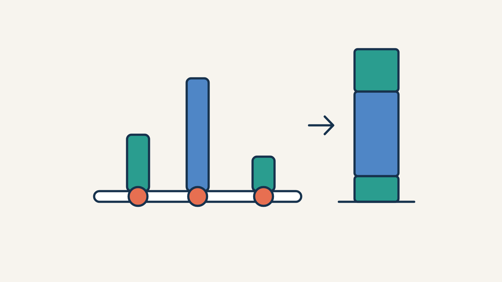
The pure premium is claim frequency times mean claim size, . That follows from three assumptions about means, not from any distribution. The distributions come in afterwards, one per part: Poisson for how many claims, gamma for how large, and Tweedie, their compound, for the total. On the French motor portfolio freMTPL2 each describes the shape of the data poorly and the mean well enough, which is all a GLM needs. The one assumption that fails is hidden in the Tweedie model: with power and a constant dispersion, it puts 70% of every relativity, on the log scale, into claim size. In the data, pure premiums differ by a factor of 4.2 across segments and claim sizes by 1.3: about 10%. Fitting frequency and severity apart drops that constraint, and uses each claim rather than each policy’s total.
First of four posts on pricing freMTPL2, followed by large claims, the model comparison and the pipeline.
What we price
freMTPL2 is a French motor third-party liability portfolio from one accounting year: 678,013 policies with their claim amounts. Each policy has risk features (driver age, bonus-malus, vehicle age, power, brand and fuel, population density, region), an exposure , the fraction of the year it was in force, and claims of amounts with total . Before anything else, a block of 9,387 policies at the top of the file goes: all of them have claims, nearly all without an amount, so they are no sample of the portfolio.
The quantity to price is the pure premium, the expected claim cost per policy-year,
One policy over its exposure: how many claims arrive, and how large each is.
The decomposition
Three assumptions
Drop the index and fix one policy’s . Its claims are the first of a sequence of potential amounts , so , and if . Assume, for some functions of the features,
- (A1) claims scale with exposure: ;
- (A2) claim sizes don’t depend on exposure: for every ;
- (A3) how many claims and how large they are are independent: .
The derivation
Condition on the number of claims first. On ,
so . Then average over :
This is Wald’s identity for the collective risk model: the pure premium is claim frequency per year times mean claim size. Two things follow.
- No distribution is needed. Only means and (A3). Poisson, gamma and Tweedie enter later, for the variance and the loss a model minimises, not for what it estimates.
- Exposure is not a feature. The last line holds for every , so is a function of alone, and enters a model only as a weight or a offset, the standard treatment in tariff GLMs. The premium is quoted for a year before anyone knows when the contract will end.
Where (A1) fails
(A1) says a policy in force for half a year expects half the claims of a full year. Short contracts claim more than that:
Claims per policy-year by exposure band, relative to the whole portfolio, with the policy-years in each band below.
Short contracts are often contracts that ended because of a claim: the car was written off, the contract cancelled. Exposure is then a consequence of the claim, not a cause, and a model that used it as a feature would price every new policy like the contracts that survived the year. So exposure stays out of , and the excess on short contracts stays a known limitation of the decomposition.
One distribution per part
A GLM estimates the mean from two things: the link and the variance function , with . The full density never enters the estimating equations. So the question for each family below isn’t whether it describes the data, but whether its variance function does. Each is compared with 534,883 training policies and their 20,879 claims, without any features, and claims are capped at 18,000 (the second post explains why).
| Poisson | Gamma | Tweedie, | |
|---|---|---|---|
| models | claim count | claim size | pure premium |
Poisson: how many
Why. If claims arrive independently at a constant rate per year, the count over years is exactly Poisson with mean . Exposure enters as the offset , with no parameter to estimate: (A1) is built in.
Training policies by number of claims, observed and under a Poisson with one common rate of 0.074 claims per policy-year, each policy with its own exposure.
How well. The bulk fits: 515,206 policies without a claim against 514,592 expected. The tail doesn’t: 1,087 policies with two or more claims against 575. Some of that is the features, which give each policy its own ; the rest is overdispersion, . Overdispersion widens the standard errors, but the Poisson score equations need only the mean, so the estimate of stays consistent. A negative binomial would fit the tail better and estimate the same means.
Gamma: how large
Why. Claim sizes are positive and right-skewed, and under the gamma their standard deviation is proportional to their mean: a segment whose claims are twice as large has claims twice as spread, so a relativity is a change of scale. Its deviance depends on only, so a few large claims don’t dominate the fit as they would under least squares.
How well. The shape fits badly. The moment estimate makes the gamma put 19% of the claims below about 100, where 6.9% are observed; it has no room for the spike of flat-rate settlements in the middle, and its exponential tail is too light, which is one more reason to cap. The variance function holds, which is what the GLM uses: across 68 one-way groups (levels of each feature, deciles of the numeric ones), the coefficient of variation stays between 1.15 and 1.65, around the portfolio’s .
Tweedie: the total
Put the two together: given and ,
then has a point mass at zero and a continuous positive part, and by the law of total variance, , so
That is the Tweedie family with power and exposure as prior weight: one model for directly, zeros included. The gamma shape fixes the power: gives , and is used throughout. The zeros fit: 96.32% of training policies have no claim, the compound model expects 96.21%.
What a single Tweedie model assumes
The derivation hides an assumption. A Tweedie GLM has one dispersion for all policies, and above depends on through . Holding it constant ties claim size to frequency:
So a single Tweedie model splits every relativity between frequency and claim size in fixed proportions: at , 30% of it, on the log scale, is frequency and 70% claim size. A segment that costs twice the average should have claims times as large. The 68 one-way groups say otherwise:
Capped pure premium against mean capped claim size per one-way group of the training data, log scales with the same factor per unit on both axes; dashed, the slope a single Tweedie model with assumes.
- Segments differ in frequency. Pure premiums range from 75 to 312 per policy-year, a factor of 4.2; mean claim sizes from 1,409 to 1,890, a factor of 1.3. Regressed on each other on the log scale, claim size has slope 0.1, not 0.7.
- Bonus-malus shows it most. From the best class to the worst, the pure premium rises by a factor of 3.8 and the mean claim size by 1.10. Bonus-malus moves only with a policyholder’s own claims, so it measures how often they claim, not how much.
- The variance agrees. If claim size is flat, grows like , not . Across the same groups the weighted variance of the pure premium grows with slope 1.21: much closer to one.
What does the wrong constraint cost? Not consistency: the Tweedie score equations, like the Poisson ones, need only the mean, so the estimate of still converges to the right thing. It weights segments by the wrong variance, so it uses the data less efficiently: it trusts expensive segments too little.
Same target, more data
Fitting frequency and severity apart drops the constraint, and it does more. A policy shows more than its total : also its count and each amount . alone can’t tell one large claim from two medium ones. Under (A3), with sizes iid given , their joint density factorises:
So the log-likelihood is a sum of a term in and a term in , maximised separately: from the counts of all policies, a Poisson GLM with offset ; from the individual amounts of the policies with claims, a gamma GLM; and by Wald’s identity. A Tweedie model collapses the observations of each policy into one number before fitting; the split collapses them only at the end.
In the model comparison, that helps the boosted trees and not the GLMs. Poisson × gamma XGBoost beats Tweedie XGBoost by 0.17 points of explained deviance, while the Poisson × gamma GLM trails the Tweedie GLM by 0.24. The likely reason is the flat claim size: the gamma GLM spends a full set of coefficients on a signal that is barely there, and its noise multiplies into every premium, while the trees stop early on the severity part and leave it nearly flat. In both the winner and the data, the tariff is a frequency model with a claim size attached.
The order of the argument
The decomposition comes first and needs only means. The distributions come second, each chosen for its variance function, each wrong about the shape of the data and right enough about the mean. And the useful question about a model is not which family it uses but what it assumes about how the parts move together: a single Tweedie model answers that question before seeing the data, and on freMTPL2 it answers it wrong.