From Kernel Regression to Self-Attention: A Line-by-Line Derivation

I have a mathematics background, and kernel regression is something I have studied deeply as part of advanced statistics.

Self-attention, on the other hand, felt slippery to me when I started learning it. It is confusing that the input tokens $\boldsymbol{x}$ play so many roles at once: they are queries, keys, and values.

If you happen to have the same background — comfortable with kernel regression, uncertain about attention — this post is for you. Following §15.4.2 and §15.5 of Kevin P. Murphy’s Probabilistic Machine Learning: An Introduction, I will derive self-attention from kernel regression step by step. I keep Murphy’s notation where possible so the post can be read alongside the book.

---

1. Kernel regression

Suppose we have $n$ training pairs $(\boldsymbol{x}_1, y_1), \ldots, (\boldsymbol{x}_n, y_n)$ with $\boldsymbol{x}_i \in \mathbb{R}^d$ and $y_i \in \mathbb{R}$, and we want to predict $y$ at a new test point $\boldsymbol{x}$. The Nadaraya–Watson estimator says: take a weighted average of the training labels, where the weight given to $y_i$ depends on how similar $\boldsymbol{x}$ is to $\boldsymbol{x}_i$:

$$f(\boldsymbol{x}) = \sum_{i=1}^{n} \alpha_i(\boldsymbol{x},\, \boldsymbol{x}_{1:n})\, y_i \tag{1}$$

Here $\alpha_i(\boldsymbol{x}, \boldsymbol{x}_{1:n}) \geq 0$ are weights that sum to one (for any fixed $\boldsymbol{x}$). A standard way to build them is to start from a density kernel. We will use the Gaussian:

$$\mathcal{K}_\sigma(u) = \frac{1}{\sqrt{2\pi\sigma^2}}\, \exp\!\left(-\frac{u^2}{2\sigma^2}\right) \tag{2}$$

where $\sigma$ is called the bandwidth. We build the weights $\alpha_i$ by normalizing the kernel across training points. Because of the normalization, the prefactor $1/\sqrt{2\pi\sigma^2}$ is irrelevant and we drop it:

$$\alpha_i(\boldsymbol{x}, \boldsymbol{x}_{1:n}) = \frac{\exp\!\left(-\dfrac{\|\boldsymbol{x} - \boldsymbol{x}_i\|^2}{2\sigma^2}\right)}{\sum_{j=1}^n \exp\!\left(-\dfrac{\|\boldsymbol{x} - \boldsymbol{x}_j\|^2}{2\sigma^2}\right)} \tag{3}$$

Recall the softmax:

$$\operatorname{softmax}_i(s_1, \ldots, s_n) = \frac{e^{s_i}}{\sum_{j=1}^n e^{s_j}} \tag{4}$$

Comparing (3) with (4), the weights are exactly a softmax — applied to the exponent of the Gaussian, not to its value. We give that exponent a name. Define the attention score

$$a(\boldsymbol{x}, \boldsymbol{x}_i) = -\frac{\|\boldsymbol{x} - \boldsymbol{x}_i\|^2}{2\sigma^2} \tag{5}$$

With this, (3) becomes

$$\alpha_i(\boldsymbol{x}, \boldsymbol{x}_{1:n}) = \operatorname{softmax}_i\!\left(a(\boldsymbol{x}, \boldsymbol{x}_1),\, \ldots,\, a(\boldsymbol{x}, \boldsymbol{x}_n)\right) \tag{6}$$

---

2. From kernel regression to a generic similarity

Substituting (6) into (1) gives

$$f(\boldsymbol{x}) = \sum_{i=1}^{n} \operatorname{softmax}_i\!\left(a(\boldsymbol{x}, \boldsymbol{x}_1),\, \ldots,\, a(\boldsymbol{x}, \boldsymbol{x}_n)\right)\, y_i \tag{7}$$

This is still pure kernel regression — we have only rewritten it. Now observe that the Gaussian score in (5) plays one specific role here: it measures how similar $\boldsymbol{x}$ is to each $\boldsymbol{x}_i$. Nothing in the structure of (7) forces that particular choice. Letting $a(\boldsymbol{x}, \boldsymbol{x}_i)$ refer to a generic similarity score — not just the Gaussian one — gives

$$f(\boldsymbol{x}) = \sum_{i=1}^{n} \operatorname{softmax}_i\!\left(a(\boldsymbol{x}, \boldsymbol{x}_1),\, \ldots,\, a(\boldsymbol{x}, \boldsymbol{x}_n)\right)\, y_i \tag{8}$$

Equations (7) and (8) look identical — and that is the point. Only the meaning of $a$ has widened: in (7) it is fixed to the Gaussian form (5); in (8) it is any real-valued function. No modelling power has been added; the similarity function has become a pluggable component. That small abstraction is what opens the door to the attention vocabulary.

---

3. Naming the pieces: queries, keys, values

We rename the objects to match standard attention notation:

Kernel regression	Attention	Role
Test point $\boldsymbol{x}$	Query $\boldsymbol{q}$	What we are predicting at
Training input $\boldsymbol{x}_i$	Key $\boldsymbol{k}_i$	What the query is compared against
Training label $y_i$	Value $\boldsymbol{v}_i$	What gets averaged into the output

With this renaming, (8) becomes

$$\operatorname{Attn}\!\left(\boldsymbol{q},\, \{(\boldsymbol{k}_i, \boldsymbol{v}_i)\}_{i=1}^n\right) = \sum_{i=1}^n \operatorname{softmax}_i\!\left(a(\boldsymbol{q}, \boldsymbol{k}_1),\, \ldots,\, a(\boldsymbol{q}, \boldsymbol{k}_n)\right) \boldsymbol{v}_i \tag{9}$$

This is mostly a rename: $\boldsymbol{k}_i = \boldsymbol{x}_i$ and $\boldsymbol{v}_i = y_i$. The split earns its keep in §8, where learned projections will let keys and values diverge.

---

4. From Gaussian scores to dot-product scores

The Gaussian score in (3) involves a squared distance. Expand it:

$$-\frac{\|\boldsymbol{q} - \boldsymbol{k}_i\|^2}{2\sigma^2} = -\frac{\|\boldsymbol{q}\|^2}{2\sigma^2} \;+\; \frac{\boldsymbol{q}^\top \boldsymbol{k}_i}{\sigma^2} \;-\; \frac{\|\boldsymbol{k}_i\|^2}{2\sigma^2} \tag{10}$$

The first term $-\|\boldsymbol{q}\|^2/(2\sigma^2)$ does not depend on $i$. To see why such a term vanishes, note that for any constant $c$ independent of $i$,

$$\operatorname{softmax}_i(s_1 + c, \ldots, s_n + c) = \frac{e^{s_i + c}}{\sum_j e^{s_j + c}} = \frac{e^c\, e^{s_i}}{e^c \sum_j e^{s_j}} = \operatorname{softmax}_i(s_1, \ldots, s_n) \tag{11}$$

so adding an $i$-independent constant to every score leaves the weights unchanged. The $-\|\boldsymbol{q}\|^2/(2\sigma^2)$ term is exactly such a constant and drops out. If we additionally assume keys are unit-norm, the third term $-\|\boldsymbol{k}_i\|^2/(2\sigma^2)$ is also constant and drops out. What remains is a softmax-equivalent score — call it $\tilde{a}$:

$$\tilde{a}(\boldsymbol{q}, \boldsymbol{k}_i) = \frac{\boldsymbol{q}^\top \boldsymbol{k}_i}{\sigma^2} \tag{12}$$

Because $\operatorname{softmax}_i(a(\boldsymbol{q}, \boldsymbol{k}_i)) = \operatorname{softmax}_i(\tilde{a}(\boldsymbol{q}, \boldsymbol{k}_i))$ for all $i$, we can replace $a$ with $\tilde{a}$ in (9) without changing any attention weight. This is the dot-product attention score. The bandwidth $\sigma$ is still a free parameter; §5 determines its standard value.

---

5. Scaling: why divide by $\sqrt{d}$

In practice $\sigma^2 = \sqrt{d}$, where $d$ is the dimension of the query and key vectors, so the score (12) becomes $\tilde{a}(\boldsymbol{q}, \boldsymbol{k}_i) = \boldsymbol{q}^\top \boldsymbol{k}_i / \sqrt{d}$. The reason is statistical. Suppose the components of $\boldsymbol{q}$ and $\boldsymbol{k}_i$ are independent, with mean zero and unit variance. Each product term $q_\ell\, k_{i,\ell}$ is then also mean-zero, with

$$\operatorname{Var}(q_\ell\, k_{i,\ell}) = \mathbb{E}[q_\ell^2]\, \mathbb{E}[k_{i,\ell}^2] = 1$$

Independence across $\ell$ means the variance of the sum is the sum of variances:

$$\operatorname{Var}(\boldsymbol{q}^\top \boldsymbol{k}_i) = \operatorname{Var}\!\left(\sum_{\ell=1}^d q_\ell\, k_{i,\ell}\right) = \sum_{\ell=1}^d \operatorname{Var}(q_\ell\, k_{i,\ell}) = d$$

So the raw dot product has standard deviation $\sqrt{d}$ — it grows with dimension. Without rescaling, large-magnitude inputs push the softmax into a saturated regime where one score dominates and gradients with respect to the others vanish. Setting $\sigma^2 = \sqrt{d}$ keeps the score variance at $O(1)$ independent of $d$, keeping the softmax in a well-behaved regime.

---

6. Matrix form

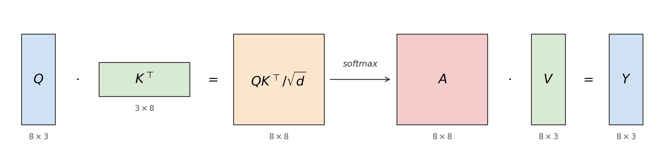
We now have all three ingredients: a softmax (6), a dot-product score $\tilde{a}$ (12), and a $1/\sqrt{d}$ rescaling. The whole pipeline vectorizes cleanly: stack the $n$ queries, keys, and values as rows of matrices:

$$Q = \begin{pmatrix} \boldsymbol{q}_1^\top \\ \vdots \\ \boldsymbol{q}_n^\top \end{pmatrix}, \quad K = \begin{pmatrix} \boldsymbol{k}_1^\top \\ \vdots \\ \boldsymbol{k}_n^\top \end{pmatrix}, \quad V = \begin{pmatrix} \boldsymbol{v}_1^\top \\ \vdots \\ \boldsymbol{v}_n^\top \end{pmatrix} \quad \in \mathbb{R}^{n \times d}$$

Then $QK^\top$ is an $n\times n$ matrix whose $(i,j)$ entry is exactly the dot-product score $\tilde{a}(\boldsymbol{q}_i, \boldsymbol{k}_j) = \boldsymbol{q}_i^\top\boldsymbol{k}_j$. To see this concretely, consider $n = 3$ tokens and $d = 2$:

$$QK^\top = \begin{pmatrix} q_{11} & q_{12} \\ q_{21} & q_{22} \\ q_{31} & q_{32} \end{pmatrix} \begin{pmatrix} k_{11} & k_{21} & k_{31} \\ k_{12} & k_{22} & k_{32} \end{pmatrix} = \begin{pmatrix} \boldsymbol{q}_1^\top\boldsymbol{k}_1 & \boldsymbol{q}_1^\top\boldsymbol{k}_2 & \boldsymbol{q}_1^\top\boldsymbol{k}_3 \\ \boldsymbol{q}_2^\top\boldsymbol{k}_1 & \boldsymbol{q}_2^\top\boldsymbol{k}_2 & \boldsymbol{q}_2^\top\boldsymbol{k}_3 \\ \boldsymbol{q}_3^\top\boldsymbol{k}_1 & \boldsymbol{q}_3^\top\boldsymbol{k}_2 & \boldsymbol{q}_3^\top\boldsymbol{k}_3 \end{pmatrix}$$

Row $i$ holds all the scores that query $i$ assigns to every key. Scaling by $1/\sqrt{d}$ and applying softmax row-wise turns each row into a probability distribution — the attention weights for that query. Multiplying by $V$ then takes a weighted average of the value rows for each query, giving the output matrix $Y \in \mathbb{R}^{n \times d}$. This is exactly (9) computed for all queries at once:

$$Y = \operatorname{Attn}(Q, K, V) = \operatorname{softmax}\!\left(\frac{Q K^\top}{\sqrt{d}}\right) V \tag{13}$$

This is scaled dot-product attention — the exact formula from “Attention Is All You Need” [Vaswani et al., 2017]. Read left to right, the pipeline has a clear shape:

The $i$-th row of $Y$ is the output for query $i$: a context-weighted blend of all the values, where the weights are determined by how well query $i$ matches each key.

---

7. Self-attention

So far we have been in the kernel-regression setting: each training point came with a scalar label $y_i$, and the value in (9) was $\boldsymbol{v}_i = y_i$. A Transformer processes something different — a sequence of tokens $\boldsymbol{x}_1, \ldots, \boldsymbol{x}_n$ with no labels attached. There are no $y_i$‘s. Every position has to supply its own payload.

The natural move is to let each token play all three roles. In self-attention, every position attends to every other position in the same sequence, using the tokens themselves for queries, keys, and values:

$$\boldsymbol{y}_i = \operatorname{Attn}\!\left(\boldsymbol{x}_i,\; \{(\boldsymbol{x}_j, \boldsymbol{x}_j)\}_{j=1}^{n}\right) \tag{14}$$

Each token $\boldsymbol{x}_i$ acts simultaneously as a query (asking “who is relevant to me?”) and contributes a key and value (answering “here is what I offer to others”). This lets the model build context-dependent representations: the embedding of the word it can depend on whether the surrounding sentence is about an animal or a street. And because there are no recurrences, all $n$ outputs $\boldsymbol{y}_1, \ldots, \boldsymbol{y}_n$ can be computed in parallel — this is what makes Transformers so much faster to train than RNNs.

---

8. Making it parametric: learned projections

To let keys and values carry different information — and more broadly, to let the model learn what aspects of each token to match on and return — introduce three learned linear projections:

$$\boldsymbol{q} = W^{(q)} \boldsymbol{x}, \quad \boldsymbol{k} = W^{(k)} \boldsymbol{x}, \quad \boldsymbol{v} = W^{(v)} \boldsymbol{x} \tag{15}$$

Each input $\boldsymbol{x}$ is passed through three different matrices before entering the attention formula. The matrices $W^{(q)}, W^{(k)}, W^{(v)}$ are learned end-to-end by backpropagation. Plugging (15) into (14) gives the full self-attention layer used in Transformers:

$$\boldsymbol{y}_i = \operatorname{Attn}\!\left(W^{(q)} \boldsymbol{x}_i,\; \left\{\left(W^{(k)} \boldsymbol{x}_j,\; W^{(v)} \boldsymbol{x}_j\right)\right\}_{j=1}^{n}\right) \tag{16}$$

This is the step that turns nonparametric kernel regression into a trained attention mechanism. The key/value split from §3 now earns its keep: because $W^{(k)}$ and $W^{(v)}$ are independent matrices, a token can be matched on one aspect of itself and return another.

---

Summary

The full derivation in one view:

$$\begin{aligned} & \underbrace{f(\boldsymbol{x}) = \sum_i \alpha_i(\boldsymbol{x}, \boldsymbol{x}_{1:n})\, y_i}_{\text{kernel regression}} \\[4pt] \xrightarrow{\text{Gaussian kernel}} \quad & \underbrace{\sum_i \operatorname{softmax}_i\!\left(-\tfrac{\|\boldsymbol{x} - \boldsymbol{x}_i\|^2}{2\sigma^2}\right) y_i}_{\text{nonparametric attention}} \\[4pt] \xrightarrow{\text{generalize similarity, rename}} \quad & \underbrace{\sum_i \operatorname{softmax}_i\!\left(a(\boldsymbol{q}, \boldsymbol{k}_i)\right) \boldsymbol{v}_i}_{\text{general attention}} \\[4pt] \xrightarrow{\text{expand, drop constants, set }\sigma^2=\sqrt{d}} \quad & \underbrace{\operatorname{softmax}\!\left(\tfrac{Q K^\top}{\sqrt{d}}\right) V}_{\text{scaled dot-product}} \\[4pt] \xrightarrow{\text{sequence attends to itself}} \quad & \underbrace{\boldsymbol{y}_i = \operatorname{Attn}(\boldsymbol{x}_i, \{(\boldsymbol{x}_j, \boldsymbol{x}_j)\}_j)}_{\text{self-attention (keys = values)}} \\[4pt] \xrightarrow{\text{learned projections}} \quad & \underbrace{\boldsymbol{y}_i = \operatorname{Attn}(W^{(q)} \boldsymbol{x}_i, \{(W^{(k)} \boldsymbol{x}_j, W^{(v)} \boldsymbol{x}_j)\}_j)}_{\text{Transformer self-attention}} \end{aligned}$$

Self-attention is not a mysterious black box. It is the natural result of applying a Gaussian similarity kernel, normalizing with softmax, generalizing the similarity, letting a sequence attend to itself, and adding learned projections to rescue the key/value distinction. Every piece has a reason.

---

Primary reference: Kevin P. Murphy, “Probabilistic Machine Learning: An Introduction”, MIT Press (2022). The kernel-regression-as-attention framing is developed in §15.4.2 (pp. 520–521); self-attention and the transformer architecture are covered in §15.5–15.5.2 (pp. 526–527). Available online at probml.github.io/pml-book/book1.html. Original transformer paper: Vaswani et al., “Attention Is All You Need”, NeurIPS 2017.