---
title: "Mutational signature estimation with Hierarchical Dirichlet Process"
pubDate: 2024-09-15T00:00:00.000Z
updatedDate: 2024-09-15T00:00:00.000Z
tags:
- Science
math: true
image: /images/blog/mutational-signature-with-hierarchical-dirichlet-process/featured.png
---
The Hierarchical Dirichlet Process (HDP) is a popular and elegant model that has gained traction in various fields, including cancer genomics. While researching methods for mutational signature estimation, I noticed that several studies employed HDPs for this purpose. However, many of these studies were published in biological journals and often lacked detailed explanations of how HDPs can be effectively applied to mutational signature estimation.
Nicola Roberts' [dissertation](https://doi.org/10.17863/CAM.22674) includes some descriptions of the mathematical model in the appendix, but even these are not fully comprehensive. In this blog post, I aim to bridge this gap by introducing the problem of mutational signature estimation using HDPs in a mathematically rigorous manner. I will begin by discussing a simpler mixture component model for mutational signatures, then explore the Dirichlet Process model, and finally delve into the Hierarchical Dirichlet Process model.
## Introduction
A key characteristic of cancer is the elevated mutation rate in somatic cells. Recognizing the patterns of somatic mutations in cancer is essential for understanding the underlying mechanisms that drive the disease (Fischer et al., 2013). This knowledge is crucial for advancing cancer treatment and prevention.
One type of somatic mutation is the single nucleotide variant (SNV), also referred to as a single base substitution. This involves the replacement of one base pair in the genome with another. There are six possible base pair mutations: C:G\>A:T, C:G\>G:C, C:G\>T:A, T:A\>A:T, T:A\>C:G, and T:A\>G:C. When considering the context of the immediate 5' and 3' neighboring bases, the total number of mutations increases to 96, calculated as $6 \times 4 \times 4 = 96$. These are known as trinucleotide mutation channels. Examples of such mutations include ACA:TGT\>AAA:TTT and ACT:TGA\>AGT:TCA. For simplicity, we will abbreviate these mutations as ACA\>AAA and ACT\>AGT respectively.
## Mutational Signature
A mutational signature $\theta$ with respect to trinucleotide mutation channels is a discrete probability distribution over the 96 mutational channels i.e. $\theta\in \Delta^{96}$ where
$$
\Delta^{n} = \left\{ (x_1, x_2, \ldots, x_{n}) \in \mathbb{R}^{n} \mid x_i \geq 0 \text{ for all } i \text{ and } \sum_{i=1}^{n} x_i = 1 \right\}.
$$
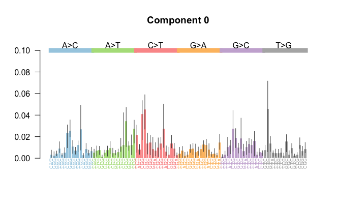
A mutational signature $\theta$ can be visualised as in the following.
The framework for studying somatic mutations through mutational signatures was introduced in a landmark study by Alexandrov et al. (2013), where over 7,000 bulk-sequenced cancer samples were analyzed. Conceptually, a mutational signature represents a biological process acting on the genome, leaving a distinct imprint captured in a probability vector, $\theta$. A comprehensive list of mutational signatures and their proposed underlying biological processes is available through the [COSMIC project](https://cancer.sanger.ac.uk/signatures/sbs/). Some of the mutational signatures and their associated probability vectors $\theta$ in the COSMIC project are consistently identifiable across most examined cohorts and signature identification algorithms [(cite)](https://pubmed.ncbi.nlm.nih.gov/34316057/).
To estimate mutational signatures and their activities, [Alexandrov et al.](https://pubmed.ncbi.nlm.nih.gov/23318258/) employed Non-Negative Matrix Factorization (NMF). NMF and its variations remain the most widely used methods for estimating mutational signatures and mutational signature activities.
## Dirichlet Process (DP)
A key mathematical tool for our study is the Dirichlet Process (DP). Formally, the Dirichlet process, denoted as $\mathrm{DP}(\alpha, H)$, is a distribution over probability measures. When we sample $G \sim \mathrm{DP}(\alpha, H)$, we obtain a probability measure $G$. The Dirichlet Process has two parameters: the concentration parameter $\alpha>0$, and the base measure $H$. The support of $G$ is a subset of the support of the base measure $H$.
To sample from the Dirichlet process, we begin by drawing an infinite sequence of i.i.d. samples $\tilde{\theta}_1, \tilde{\theta}_2, \ldots \sim H$. Then, we draw a vector $\boldsymbol{e} = \{e_1, e_2, \ldots\} \sim \operatorname{Stick}(\alpha)$, where $\operatorname{Stick}(\alpha)$ refers to the stick-breaking process. Intuitively, the stick-breaking process works by repeatedly breaking off and discarding a random fraction of a "stick" that is initially of length $1$. Each broken off part of the stick has a length $e_k$. The stick-breaking process generates a sequence $\boldsymbol{e} \in \Delta^\infty$, where the total length of all the broken pieces is 1.
Finally, we construct the random measure $G$ as:
$$G = \sum_{k=1}^{\infty} e_k \delta_{\tilde{\theta}_k}$$
where $\delta_{\tilde{\theta}_k}$ is a Dirac delta function centered at $\tilde{\theta}_k$. The resulting measure $G$ is discrete, with countable support given by $\{\tilde{\theta}_1, \tilde{\theta}_2, \ldots\}$.
### Mathematical properties of Dirichlet Process
The base measure $H$ serves as the mean of the random measure $G$. Specifically, for any measurable set $A$, the expectation of $G(A)$ under the Dirichlet process is given by \[@millerDirichletProcessModels\]:
$$
\mathrm{E}_{G \sim \mathrm{DP}(\alpha, H)}[G(A)]=H(A)
$$
As $\alpha \rightarrow \infty$, the distribution of $G$ converges to $H$ in the weak topology, meaning that larger values of $\alpha$ make $G$ more closely resemble the base measure $H$.
In summary, $G$ is centered around the prior distribution $H$, with the concentration parameter $\alpha$ controlling how tightly $G$ clusters around $H$. A higher $\alpha$ reduces variability, causing $G$ to approximate $H$ more closely.
### References
Recommended material for Dirichlet Process
- https://en.wikipedia.org/wiki/Dirichlet_process
- https://www.geeksforgeeks.org/dirichlet-process-mixture-models-dpmms/
- https://towardsdatascience.com/dont-be-afraid-of-nonparametric-topic-models-d259c237a840
- https://pawel-czyz.github.io/posts/dirichlet-process.html
NoteBook Impelementation of the Dirichlet Process
- https://datamicroscopes.github.io/ncluster.html
- https://github.com/tdhopper/notes-on-dirichlet-processes/tree/master
- https://github.com/tdhopper/notes-on-dirichlet-processes/blob/master/pages/2015-07-28-dirichlet-distribution-dirichlet-process.ipynb
## Modelling mutational signature with DP
Dirichlet processes have been utilized in previous studies to model trinucleotide mutations associated with mutational signatures [(cite)](https://doi.org/10.17863/CAM.22674) and [(cite)](https://www.nature.com/articles/s41586-019-1913-9). Although Appendix B (p. 234) and Chapter 4 (p. 132) in [(cite)](https://doi.org/10.17863/CAM.22674) provide a mathematical overview of the model, they lack sufficient detail and are not fully comprehensive. This section aims to address that gap by deriving the Dirichlet Process model for trinucleotide mutations in a thorough and accessible manner. We will begin by introducing a more intuitive approach to modeling trinucleotide mutations using a mixture model. To illustrate, consider the trinucleotide mutations within a single sample, which can be encoded as $x \in \{1, \ldots, 96\}$, representing the 96 possible trinucleotide mutation types.
#### Step 1: Known number of mutational signatures $K$
Let's begin by assuming we know the number of active mutational signatures, denoted as $K$. Each signature is represented by a discrete probability distribution, $\tilde{\theta}_k \in \Delta^{96}$, where $k=1, \ldots, K$. Since we assume that we have no prior knowledge of the specific mutational signatures, we model these distributions as:
$$
\begin{aligned}
\tilde{\theta}_k & \sim \operatorname{Dir}\left(\frac{1}{96} \cdot \mathbf{1}_{96}\right)
\text{ for } k=1,\ldots, K\\
\end{aligned},
$$
where $\operatorname{Dir}$ denotes the Dirichlet distribution, serving as a symmetric prior. Similarly, we assume no prior information about the activity of these mutational signatures. We model the activity of the $K$ mutational signatures $\boldsymbol{e} \in \Delta^K$ in a sample as:
$$
\begin{aligned}
\boldsymbol{e} \mid \alpha,K & \sim \operatorname{Dir}\left(\frac{\alpha}{K} \cdot \mathbf{1}_K\right).
\end{aligned}
$$
where $\alpha$ is a hyperparameter controlling the concentration of the distribution. Next, let $z_i=k$ represent the event that the $i$-th mutation was generated by the $k$-th mutational signature. If we observe a total of $M$ trinucleotide mutations in our sample, we draw each $z_i\in \{\{1,\ldots, K\}\}$ according to the mutational signature activity $\boldsymbol{e}$, as follows:
$$
\begin{aligned}
z_i \mid \boldsymbol{e} & \sim \operatorname{Categorical} \left(\boldsymbol{e}\right) \text{ for } i=1,\ldots, M,
\end{aligned}
$$
indicating that the probability $\mathrm{P}\left(z_i=k\right)=e_k$, where $e_k$ is the activity level of signature $k$. Finally, the observed trinucleotide mutation $x_i \in\{1, \ldots, 96\}$ is drawn from a categorical distribution based on the corresponding mutational signature $z_i=k$ and its distribution $\tilde{\theta}_k$ :
$$
\begin{aligned}
\{{1,\ldots, 96}\} \ni x_i \mid z_i=k, \tilde{\theta}_k & \sim \operatorname{Categorical} \left(\tilde{\theta}_{k}\right) \text{ for } i=1,\ldots, M
\end{aligned}
$$
This completes our model, which describes how the mutational signatures $\left\{\tilde{\theta}_1, \ldots, \tilde{\theta}_K\right\}$ generate the observed trinucleotide mutations $\left\{x_1, \ldots, x_M\right\}$
##### Graphical model for known number of components $K$
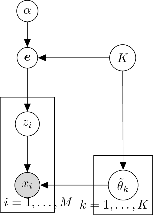
We can visualize the process that generates trinucleotide mutations in a sample using a graphical model:
Here the grey background color indicates that $x_i$ is an observed random variable.
#### Step 2: Equivalent model as mixture
In the next step, we aim to integrate out the indicator variable $z_i=k$ in our model, seeking a different representation of the same model. As before, we draw the mutational signature activities as follows:
$$
\begin{aligned}
\boldsymbol{e} \mid \alpha,K & \sim \operatorname{Dir}\left(\frac{\alpha}{K} \cdot \mathbf{1}_K\right).
\end{aligned}
$$
Let $H=\operatorname{Dir}\left(\frac{1}{96} \cdot \mathbf{1}_{96}\right)$. Similar to the last step, we generate the mutational signatures as
$$
\begin{aligned}
\tilde{\theta}_k & \sim H \text{ for } k=1,\ldots, K.
\end{aligned}
$$
Now, instead of assuming that each observation $i=1, \ldots, M$ is first assigned a mutational signature $z_i \in\{1, \ldots, K\}$ and then drawn from the corresponding signature $\tilde{\theta}_{z_i}$ we directly draw $\theta_i$ from $\left\{\tilde{\theta}_1, \ldots, \tilde{\theta}_K\right\}$, with probabilities $\left\{e_1, \ldots, e_K\right\}$ for each observation:
$$
\begin{aligned}
\theta_i \mid \boldsymbol{e}, \tilde{\theta}_1, \ldots \tilde{\theta}_K & \sim G=\sum_{k=1}^K e_k \delta_{\tilde{\theta}_k}\left(\theta_i\right) \text{ for } i=1,\ldots, M.
\end{aligned}
$$
Here, $G$ represents a finite mixture distribution with support on the acting mutational signatures. Finally, we draw the trinucleotide mutation as follows:
$$
\begin{aligned}
x_i \mid \theta_i & \sim \operatorname{Categorical} \left(\theta_i\right) \text{ for } i=1,\ldots, M.
\end{aligned}
$$
#### Step 3: Unknown, unbounded number of components $K$
Let
$$
\Delta^{\infty} = \left\{ (\theta_1, \theta_2, \ldots, ) \in \mathbb{R}^{\infty} \mid \theta_i \geq 0 \text{ for all } i \text{ and } \sum_{i=1}^{\infty} \theta_i = 1 \right\}.
$$
We now extend the model from the previous step to allow for an unknown number of components $K$, with any $K \in \mathbb{N}$ being possible. As in the previous step, we generate the underlying mutational signatures $\tilde{\theta}_k\in \Delta^{96}$ from $H$ as follows:
$$
\begin{aligned}
\tilde{\theta}_k & \sim H \text{ for } k=1,2,\ldots
\end{aligned}
$$
Previously, we sampled a finite set of $K$ mutational signatures $\tilde{\theta}_k$, but now we generate an infinite sequence of signatures. Accordingly, the mutational signature activities $\boldsymbol{e}$ now lie in $\Delta^{\infty}$. To model these activities, we use the Stick-breaking process, which defines a distribution over $\Delta^{\infty}$. Thus, we sample the mutational signature activities as:
$$
\begin{aligned}
\boldsymbol{e} \mid \alpha &\sim \operatorname{Stick}(\alpha).
\end{aligned}
$$
Intuitively, the stick-breaking process works by repeatedly breaking off and discarding a random fraction of a "stick" that is initially of length $1$. Each broken off part of the stick has a length $e_k$. The stick-breaking process generates a sequence $\boldsymbol{e} \in \Delta^\infty$, where the total length of all the broken pieces is $1$. Consequently, the mixture distribution $G$, which previously had finite support, now has countably infinite support $\left\{\tilde{\theta}_1, \tilde{\theta}_2, \ldots\right\}$ and takes the form:
$$
\begin{aligned}
\mathcal{P}(\Delta^{96}) \ni G&=\sum_{k=1}^{\infty} e_k \delta_{\tilde{\theta}_k}\left(\theta_i\right) ,
\end{aligned}
$$
where $\mathcal{P}(\Delta^{96})$ denotes the space of probability distributions on $\Delta^{96}$. We draw $\theta_i$ from the support of $G$, which is $\left\{\tilde{\theta}_1, \tilde{\theta}_2, \ldots\right\}$, as follows:
$$
\begin{aligned}
\theta_i \mid G & \sim G \text{ for } i=1,\ldots, M \\
\end{aligned}
$$
Finally, we observe the mutations as
$$
\begin{aligned}
\{{1,\ldots, 96}\} \ni x_i \mid \theta_i & \sim \operatorname{Categorical} \left(\theta_i\right) \text{ for } i=1,\ldots, M
\end{aligned}
$$
#### Step 4: Short hand notation
We summarize the first three lines in the last equation and say that $G$ was genereated by the Dirichlet Process $\mathrm{DP}$ with the parameters $\alpha$ and $H$. This way the above equations simplify to
$$
\begin{aligned}
G &\sim \mathrm{DP}(\alpha, H)\\
\Delta^{96}\ni \theta_i \mid G &\sim G \text{ for } i=1,\ldots, M \\
\{{1,\ldots, 96}\} \ni x_i \mid \theta_i & \sim \operatorname{Categorical} \left(\theta_i\right) \text{ for } i=1,\ldots, M
\end{aligned}
$$
This concludes our derivation of how we can model trinucleotide mutations with a Dirichlet Process, as used in [(cite)](https://www.nature.com/articles/s41586-019-1913-9). The Dirichlet Process approach presents an alternative approach to estimate mutational signature and signature activity as alternative to the classical approach based on Non-negative Matrix Factorisation used in [(cite)](https://www.nature.com/articles/nature12477).
##### Graphical Model of Dirichlet Process
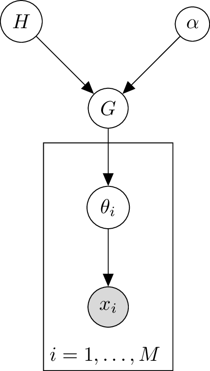
We can visualise the Dirichlet process as a graphical model:
ThegraphicalmodelofaDirichletProcess.
## Hierarchical Dirichlet Process (HDP)
By taking composition of multiple Dirichlet Processes, we obtain a Hierarchical Dirichlet Process (HDP) [(cite)](https://www.tandfonline.com/doi/abs/10.1198/016214506000000302). Recall that Dirichlet processes excel at modelling mixtures with an unknown number of components. HDPs are tailored for the situation when we have groups of mixture components and/or hierarchies between mixture components. For our model of trinucleotide mutations, we can use HDP to account for multiple samples. We expect from biology that there are general trends of mutational signature activity. However, we expect those trends to be more similar within a sample than between samples. In a mixture modelling approach, this would be captured by separate mixture models for each sample and information sharing between the weights of each sample. In the Dirichlet Process approach, this can be reflected by the HDP model. As before, we start with the prior distribution $H$. We draw a common base distribution $G_0$ from a Dirichlet Process as
$$
\begin{aligned}
G_0 &\sim \mathrm{DP}(\alpha_0, H).\\
\end{aligned}
$$
Let's assume we have $N$ samples. For each sample, we draw a seperate Dirichlet Process $G_j$ from the common base distribution $G_0$ as
$$
\begin{aligned}
G_j \mid G_0 &\sim \mathrm{DP}(\alpha_j, G_0) \text{ for } j = 1,2,\ldots N.
\end{aligned}
$$
In other words, we have a Dirichlet Process $G_0$ at the top and other Dirichlet Processes $G_j$ at the lower hierarchies. As described in the section of the mathematical properties of the Dirichlet Process, each $G_j$ will vary around $G_0$. This allows the different samples $G_j$ to share information via $G_0$. Let's assume we observe $M_j$ mutations in the $j$-th sample. We draw the mutations as before:
$$
\begin{aligned}
\theta_{j i} \mid G_j &\sim G_j \text{ for } i = 1,2,\ldots M_j , \\
x_{ji} \mid \theta_{j i} & \sim \operatorname{Categorical} \left(\theta_{j i}\right).
\end{aligned}
$$
The corresponding graphical model is:
### Estimation of mutational signature and mutational signature activity
Let's assume we have the mutational signatures $\left(\theta_k\right)_{k\in \mathbb{N}}\subset \Delta^{96}$ acting on the genome. Borrowing notation from the model with a finite number of mutational signatures, let $z_{ji}\in \mathbb{N}$ denote the mutational signature that generated the mutation $x_{ji}\in \{1,\ldots,96\}$. By fitting a HDP to our data we will obtain an estimate $\hat{z}_{ji}$ of $z_{ji}$. Our estimate $\hat{\theta}_k$ for the associated probability vector $\theta_k \in \Delta^{96}$ of mutational signature $k$ is
$$\hat{\theta}_k=\frac{\sum_{l=1}^{96}\sum_{j=1}^N\sum_{i=1}^{M_j} \mathbb{I}(\hat{z}_{ji}=k)\mathbb{I}(x_{ji}=l)\delta_l}{\sum_{j=1}^N\sum_{i=1}^{M_j} \mathbb{I}(\hat{z}_{ji}=k)},$$
where $\delta_l\in \Delta^{96}$ has mass $1$ at position $l$. Further, we estimate the mutational signature activity $e_{kj}$ of mutational signature $k$ in sample $j$ by
$$\hat{e}_{kj}=1/M_j\sum_{i=1}^{M_j} \mathbb{I}(\hat{z}_{ji}=k).$$
### Advantages of HDP approach compared to the classical NMF approach for mutational signature estimation
The Hierarchical Dirichlet Process (HDP) approach offers several advantages over the classical Non-negative Matrix Factorization (NMF) method. It allows for the incorporation of prior knowledge and the imposition of group structures, such as the expectation that certain features should behave in coordinated ways [(cite)](https://doi.org/10.17863/CAM.22674). In mutational signature analysis, two key tasks---(1) de novo discovery of mutational signatures and (2) estimation of signature activity---can be performed simultaneously using HDP. The method can match the observed mutational catalog to an existing signature library while also identifying new signatures by pseudo-counting the existing library as observational data. Additionally, HDP facilitates the direct learning of the number of signatures from the data, overcoming a common challenge in NMF, which often struggles to select the appropriate number of signatures. While some NMF variants can quantify uncertainty, HDP provides this capability more easily.
### References
Python Implementations 1
- https://radimrehurek.com/gensim/models/hdpmodel.html
- Gensim is a Python library for *topic modelling*, *document indexing* and *similarity retrieval* with large corpora. Target audience is the *natural language processing* (NLP) and *information retrieval* (IR) community.
- https://github.com/piskvorky/gensim/blob/develop/gensim/models/hdpmodel.py
- based on https://github.com/blei-lab/online-hdp
- https://towardsdatascience.com/dont-be-afraid-of-nonparametric-topic-models-d259c237a840
- https://towardsdatascience.com/dont-be-afraid-of-nonparametric-topic-models-part-2-python-e5666db347a
- https://github.com/ecoronado92/hdp
- https://github.com/morrisgreenberg/hdp-py
Python Implementations 2
- https://radimrehurek.com/gensim/models/hdpmodel.html
- Gensim is a Python library for *topic modelling*, *document indexing* and *similarity retrieval* with large corpora. Target audience is the *natural language processing* (NLP) and *information retrieval* (IR) community.
- https://github.com/piskvorky/gensim/blob/develop/gensim/models/hdpmodel.py
- based on https://github.com/blei-lab/online-hdp
- https://towardsdatascience.com/dont-be-afraid-of-nonparametric-topic-models-d259c237a840
- https://towardsdatascience.com/dont-be-afraid-of-nonparametric-topic-models-part-2-python-e5666db347a
- https://github.com/ecoronado92/hdp
- https://github.com/morrisgreenberg/hdp-py
- Simple Jupyter notebook: https://github.com/tdhopper/notes-on-dirichlet-processes/blob/master/pages/2015-07-30-sampling-from-a-hierarchical-dirichlet-process.ipynb (just for sampling?)
Recommended Material for HDP
- https://en.wikipedia.org/wiki/Hierarchical_Dirichlet_process
- https://mlg.eng.cam.ac.uk/zoubin/tut06/ywt.pdf